
Blood Test Tracker plus
Hello and thank you for your purchase! This comprehensive guide will walk you through configuring your spreadsheet, entering your historical data, and visualizing your health trends step-by-step. Feel free to watch the full video below, or use the timestamps to jump to the exact section you need.
Step-by-Step Guide
Select your version below to view specific instructions.
When you first open the file, you must click "Enable Content" or "Enable Macros". This is required for the "Duplicate Charts" button to function.
Select Date Format
First thing to do is select your desired 'Date Format' from the selector in the 🏠 HOME tab in cell 23 B:E. This dropdown controls the dates across the entire spreadsheet, except for Charts/Graphs which will remain in standard 'Month-Year' format to prevent text crowding.
Enter Personal Details
Navigate to the 🩸 Test Results tab. Input your personal details in cells A1 to H2. When you insert your Date of Birth in cell F1, your age will automatically display above each test date in row 1.
Enter Test Dates
In row 4 of the 🩸 Test Results tab, input your test dates in chronological order starting from cell I4 (oldest on the left, newest on the right).
IMPORTANT EXCEPTION: Never insert a new column to the left of Column I. Column I holds the master formulas for your auto-calculated rows. If you need to add an older date, insert a new column to the right, copy/paste your Column I data over to make room, and type your older data into Column I.
Add Reference Ranges
In columns B and C of the 🩸 Test Results tab, enter the Optimal ranges. In columns D and E, input the Laboratory reference ranges. Select the unit of measure in column F. If you do not know the optimal range you can leave it blank. Your results will simply appear in one of three colors (no turquoise).
If you need to move the biomarkers around, please do not delete or move row 5. This row serves as the starting reference point for most formulas, dropdowns, conditional formatting, and charts. You can rename items in row 5 if needed, and add or move rows below it as necessary to continue entering data.
If you need to move the biomarkers around, please do not delete or move row 5. This row serves as the starting reference point for most formulas, dropdowns, conditional formatting, and charts. You can rename items in row 5 if needed, and add or move rows below it as necessary to continue entering data.
Insert Test Results
Enter your blood test results using only numbers. Avoid using words like "positive", "negative", ">", or "<" as they disrupt the conditional formatting. For biomarkers with negative or positive values, select - (0) or + (1) as your unit of measure and input 0 for negative and 1 for positive results. For Non-Reactive or Reactive results, select NR (0) or R (1) as your unit of measure and input 0 for Non-Reactive and 1 for Reactive. If your lab does not specify a lower range (e.g., < 9) you can input 0. If your lab does not specify an upper range, you can either: 1. Request the limit from your lab, 2. Research other labs' ranges, or 3. Insert a reasonable placeholder value.
Recording Events or Notes
Use cells in row 3 located above the test dates to record significant events (e.g., hospitalization, fever, diagnosis, etc.) or notes (e.g., name of the laboratory or doctor) regarding that particular panel of tests. When text is entered, the cell background automatically turns pale yellow. Use column H to record notes (e.g., ask doctor why this is still elevated) regarding particular biomarkers.
Adding a New Biomarker
Right click on the row where you want to add a new biomarker and select Insert. The conditional formatting automatically applies to new rows. Ensure you give each one a unique name so the dropdowns and any data pull-through work correctly across ⚡ Quick Stats and 📊 Charts. For example, “Glucose, Fasting" and “Glucose, Non-Fasting” rather than “Glucose” twice.
Adding a New Category
The easiest way is to copy and paste from another category or sub-category row. This is because you need to remove the unit of measure drop down from column F and replace it with either the number 1 to maintain the light blue background or number 2 to maintain the light gray formatting. To hide the 1 or 2 change the font color to match the background color.
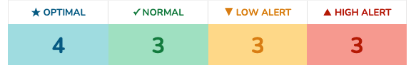
Understanding Status & Colors
The status in column G tells you if your most recent test result was optimal, normal, high, or low. The background color of the cells will automatically change to match these statuses to help you visualize trends. Values that fall within a 5% margin of the lower or upper limit will also be highlighted to warn you of borderline results.
Auto-calculated rows
To save you time, I've added pre-coded formulas that automatically calculate common ratios, HOMA-IR, T7, QUICKI, TyG, and even Levine's PhenoAge (included as a free bonus!).
Look for the lock icon (🔒 Auto) in the Notes column to spot them. These rows are fully automated—please do not type in them unless you want to override the result.
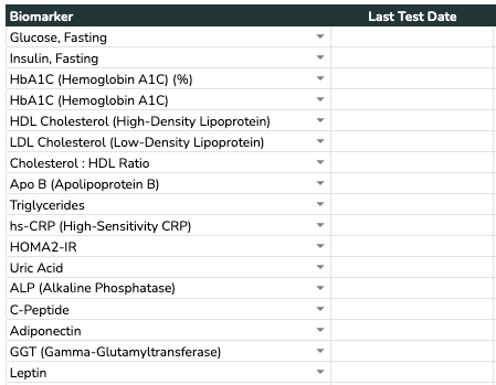
Focus on Health Goals
This tab allows you to track specific biomarker groups without altering the main 🩸 Test Results tab. Select up to 100 biomarkers using the dropdowns in columns B to C. All relevant data is automatically pulled from your 🩸 Test Results tab. You can override the formula in column F if you prefer to enter Notes manually, as opposed to pulling them from your 🩸 Test Results tab.
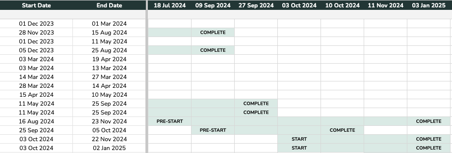
Monitor Interventions
Use the section at the top to observe how your actions (nutrition, lifestyle, or medical) influence trends over time. Click the "+" button to the left of row 5 to expand the Intervention Tracker. In columns B to E, describe your intervention (e.g., "Start a ketogenic diet", "Levothyroxine 100mcg QD"). Enter a start date in column F and the tracker will highlight the timeline in light blue to show when the intervention is active. Once completed, add an end date in column G.
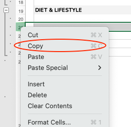
1. Go to the 'Intervention Tracker' section within the ⚡ Quick Stats tab.
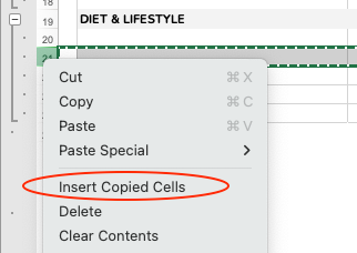
2. Right click on one of the existing rows, and select Copy.
3. Right click on the row where you want to add your new row and select Insert Copied Cells.
The formulas in columns I:DD will automatically apply to the new row.
Select Date Range
Navigate to the 📊 Charts tab. Select the time period that you want to graph by entering the start and end dates in cells R1 and T1, or tick the box in cell W1 to select all dates available.

Select Biomarkers
Use the dropdown menu embedded within the biomarker title itself (columns B to D) to select what you want to graph. The biomarker ranges will automatically populate the box below and the graphs will display the test results available within the selected time frame.
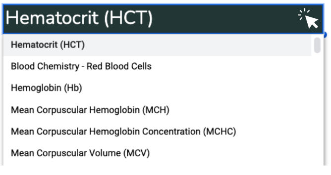
Chart Statistics
The charts automatically calculate your latest value, average value, and lowest/highest value according to the date range you have selected.
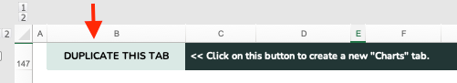
Duplicate the Chart
You can chart up to 12 biomarkers per tab. To create separate charts for different health focuses (e.g., Thyroid Health, Inflammation), you should duplicate the tab. You can also hide and unhide unused charts using the group/ungroup buttons in the left side gutter.

Ready to decode your labs?
Hi, I'm Tamara! While I love building a good spreadsheet, my primary work is in clinical practice as a Nutritional Therapist.
Now that your data is beautifully organized, you might be wondering how to interpret it. If you have recent blood tests (from the last 3 months), I can help you spot hidden imbalances and trends before they become bigger issues. You'll walk away knowing what to prioritize as well as where and how to start.
If you don't have recent blood labs and want to know my recommended panels for a functional overview of your health then download my Biomarker List below.
Knowledge Base & FAQs
Setup & Data Entry
Laboratory reference ranges are used by healthcare providers to interpret if a result falls within an expected range. These have been purposefully kept blank as there are no universally standardized reference ranges for most biomarkers; they vary by lab and region. I recommend using the specific ranges provided on your lab reports and speaking with your healthcare provider for guidance.
Standard reference ranges are established by individual laboratories based on a broad population and can often be quite wide. Conversely, optimal reference ranges are based on data from healthy populations. They are designed to identify an individual's optimal health status and look for signs of dysfunction at the cellular level, often years before it develops into a disease state.
Your birthday is included to automatically calculate your age in row 1 at the time of each blood test. This ensures your age is accurately reflected without manual calculation, allowing for better tracking of age-related health trends.
While this spreadsheet is for personal use, it may also be viewed by health professionals. These questions have been included to account for sex-specific differences (e.g., hormone levels, disease risks) and ethnic/ancestral backgrounds that may influence health outcomes. However, if you do not feel comfortable providing this information, you may leave these sections blank.
Titers are often expressed as ratios (1:10, 1:40). To graph these, you should enter the reciprocal value. For example, if your result is 1:10, enter 10. If it is 1:40, enter 40. This allows the chart to visualize the magnitude of the titer.
I usually recommend using the reference range from your most recent lab report or the lab you use most consistently. You can also insert the name of the lab above each column for clarity. If you want to track different units (e.g., MCHC in g/dL and g/L), you can add additional rows as long as they are named differently. Just bear in mind that the charts will reflect the data exactly as entered—if you keep them in separate rows, you can select and chart each lab's data separately.
Calculations & Formulas
If your lab report provides the exact number, you can simply click on the cell for that specific date and type your lab's number over the formula. It will only overwrite that specific date and won't break the rest of the sheet.
Easy! Click on an empty cell to the left or right of the one you deleted (in the same row). Click the small square in the bottom right corner of that cell's outline, and drag it over the empty cell. The formula will copy right back over.
Auto-calculated ratios and indexes require all parent values to be entered before they can calculate. For example, the AST:ALT ratio requires both your AST and ALT results to be filled in. Once all necessary data is entered for a specific date, the calculation will appear automatically.
Troubleshooting tips:
- Ensure you haven't accidentally deleted the formula in that specific cell.
- Ensure all parent values have been added for that specific date.
- Double-check that all units of measure have been selected from the dropdowns, as the smart formulas depend on these to know how to calculate for you.
Some laboratories use a simpler formula for Anion Gap that excludes Potassium: Sodium - (Chloride + Bicarbonate). This tracker uses the more comprehensive and clinically accurate formula that includes Potassium: (Sodium + Potassium) - (Chloride + Bicarbonate). Because of this, your calculated result here might be slightly higher than a lab report that excludes Potassium.
AIP is not a simple ratio. The standard clinical formula requires converting Triglycerides and HDL to mmol/L and then applying a Base-10 Logarithm: Log10(Triglycerides / HDL). The spreadsheet handles these complex unit conversions and logarithmic calculations automatically behind the scenes, which is why a simple manual division won't match the result.
Formulas like HOMA-IR and QUICKI rely on your Fasting Insulin and Fasting Glucose levels. When converting Fasting Insulin between International SI units (pmol/L) and US units (μIU/mL), different laboratories and online tools use slightly different conversion factors.
Some calculators use a rounded conversion factor of 6.0, while others use the more precise factor of 6.945. This spreadsheet uses the precise 6.945 factor to ensure maximum accuracy. As a result, you might notice a tiny decimal discrepancy compared to calculators using 6.0, but this will not affect the overall clinical interpretation of your results.
Morgan Levine, Steve Horvath, and 16 other top scientists developed a formula to calculate your phenotypic (biological) age. Their aim was to determine biological age using routine blood biomarkers, prioritizing accessibility over precision.
The 10 markers necessary for calculating this are: Albumin, Creatinine, Glucose, C-Reactive Protein (hsCRP), Lymphocyte Percent, Mean Corpuscular Volume (MCV), Red Blood Cell Distribution Width (RDW), Alkaline Phosphatase (ALP), White Blood Cell Count (WBC), and Chronological Age.
The optimal range has been set to > -5 years younger than chronological age, and normal to -5 to 0 years younger than chronological age. The Delta Age shows that difference.
If you prefer to calculate and hardcode the value yourself, you can use a free online calculator like Longevity Tools (not affiliated).
Formatting & General Tips
Right click on the row or column you want to hide and select Hide. To unhide, select surrounding cells and click Unhide.
If you have already selected your preferred date format from the dropdown on the 🏠 HOME tab but the dates still aren't displaying correctly, ensure that your Locale, Region, and Time Zone settings are accurate.
For Windows Users:
- Open the Control Panel on your computer.
- Go to Clock and Region > Region.
- Set the location to your desired region and ensure the date and time formats are correct.
For Mac Users:
- Open System Settings.
- Go to General > Language & Region.
- Ensure your Region is set correctly.
Printing Test Results:
Highlight the cells that you want to print. Go to File > Print Area > Set Print Area. Then, go to File > Print. Under the printer settings choose Print Selection. Pick the page orientation. If you have a lot of columns then Landscape will be more appropriate. Set your margins all around or select Scale to Fit if appropriate. Print.
Printing Charts:
This will yield a printout of 3 biomarkers per page (4 pages in total) in Landscape orientation.
Go to File > Print. Select Landscape from the page orientation. Select Scale to Fit. Print.
To duplicate the entire spreadsheet go to File in the menu bar, select Save As, and save a new workbook with a different name. To duplicate a single tab, within the same file, right click on the Tab name below, select Move or Copy, and check the box Create a Copy in the dialog box.
This usually means the column is too narrow to display the content. Simply double-click the right border of the column header to auto-expand it, or drag it wider.
Compatibility & Tech
I understand the desire for automation! However, because I sell these spreadsheets internationally and labs vary hugely in their PDF formats, naming conventions, and layouts, it isn't currently feasible to offer one universal "import" tool that works reliably for everyone. You will need to manually enter your data yourself, which also provides a good opportunity to review your results closely.
Unfortunately, you cannot automatically import your previous data and will need to manually add your test results into this new spreadsheet. Be careful when copying and pasting test results to avoid disrupting the conditional formatting. The safest method is to use 'Paste Without Formatting' or 'Paste as Values' (Ctrl+Shift+V on a PC or Cmd+Shift+V on a Mac).
While you can view the data on mobile devices, I strongly recommend using a desktop or laptop for data entry and analysis. The complex charts and conditional formatting are designed for a full-screen experience and may not display or function correctly on mobile versions of Excel or Google Sheets.
This limit exists to keep the complex formulas and conditional formatting fast and responsive. Additionally, charting more than 100 points at once makes the axis labels difficult to read. For users with very deep historical records, I recommend duplicating the file (for example, keeping one file per decade) to ensure the spreadsheet doesn't lag.
This spreadsheet is generally compatible with Excel 2016 and later. If you are a Mac user, please note that I use a Mac myself and built this using Office 365. Older standalone versions (like Office 2019 for Mac) may not support the full functionality.
Note on Web/Mobile: I do not recommend using Excel Online (Web Browser) or the mobile app. These versions do not support Macros, which are required in this file to reliably duplicate the charting tools, nor do they support some of the more complex formulas and charts used in this tracker. The same limitations apply to LibreOffice and Apple Numbers.
Yes, the Excel version uses a simple macro for one specific purpose: to allow you to create clean, working copies of the 📊 Charts tab with a single click. This ensures all complex charting formulas remain intact when you want to visualize different datasets.
The macro does not access the internet or modify other files. However, if you are uncomfortable enabling macros or your computer's security settings prevent them, please reach out to me. I can provide a macro-free version with 10 pre-generated chart tabs ready for you to unhide. Please note that because these tabs are pre-built, the macro-free file is slightly larger in size than the standard version.
To ensure the tracker functions smoothly and to prevent accidental deletion of complex formulas, certain areas (like the quick stat tabs and charts) have been locked. This protects the integrity of your data and ensures the charts generate correctly! Because unlocking the spreadsheet often leads to broken features that are difficult to troubleshoot, I do not provide the password to unlock the workbook. If you have a specific customization request, please reach out and I will do my best to help or consider it for a future update.
Currently, the tracker is only available in English. However, because the spreadsheet is fully customizable, many international users simply type over the English column headers and categories with their native language. If I receive enough requests for a specific language, I will certainly consider translating it in a future update.
Privacy & Sharing
Each spreadsheet is designed for one person to maintain data integrity. To track a family, simply set up one "Master" file with your preferred units and ranges, then duplicate that file for each family member.
You are welcome to share PDFs or screenshots of the charts with clients. However, to share the actual spreadsheet or use it within a program/course, a Practitioner License is required.
Version History
Introduced advanced auto-calculated metrics (HOMA-IR, QUICKI, TyG, PhenoAge, Delta Age, and various ratios). Upgraded 'Quick Stats' with latest known values and a new bonus "Longevity" Quick Stat. Enhanced the Charting area with hide/unhide functionality (Excel only) and introduced new metrics. Significantly improved UX with a universal Date Format selector, "extreme normal" conditional formatting for borderline results, data validation warnings, and the ability to safely rename the Test Results tab. Streamlined the file by moving tutorials to the website and refined Immune Health sub-categories.
Implemented a macro-based approach for duplicating the Charts tab.
Added extra biomarkers (400+) and units of measure (64). Added a 'Status' calculator and 'Notes' column. Added Anthropometry & Body Metrics, Fecal Occult Blood Test and Urinalysis. Added a Quick Stats tab with in-built intervention tracker. Added a section for personal details.
New charting tool that can track and graph up to 100 time intervals (dates/columns). Includes both bar and line graphs. Added 'Protein Electrophoresis' to categories and some extra units of measure (49).
Added extra biomarkers (300) and units of measure (43). Implemented grouping function for rows.
Enhanced charting tool for Google Sheets to ignore empty cells.
Initial release.
Disclaimer & Legal
Copyright Notice: The design and spreadsheet is original and copyrighted to EYZHN Limited. Your purchase of this product is for personal use only. Redistribution or resale is strictly prohibited, either in part or in full, with or without modifications.
Medical Disclaimer: This spreadsheet is for informational purposes only. Consult a qualified healthcare professional for medical advice. EYZHN Limited is not liable for any damages resulting from the use of this spreadsheet.
Refunds and Cancellations: This is a digital product available for instant download and all sales are final. Due to the nature of digital downloads, refunds and cancellations are not accepted.
Compatibility: This spreadsheet is designed exclusively to work with either Google Sheets or Microsoft Excel, depending which version you purchased. Neither are compatible with Apple Numbers, GoodNotes, LibreOffice or other software.
Love your new spreadsheet?
Earn 20% commission by sharing it with your community.
Join the Affiliate Program